Copyright 2018 The TensorFlow Authors.
[1]:
#@title Licensed under the Apache License, Version 2.0 (the "License");
# you may not use this file except in compliance with the License.
# You may obtain a copy of the License at
#
# https://www.apache.org/licenses/LICENSE-2.0
#
# Unless required by applicable law or agreed to in writing, software
# distributed under the License is distributed on an "AS IS" BASIS,
# WITHOUT WARRANTIES OR CONDITIONS OF ANY KIND, either express or implied.
# See the License for the specific language governing permissions and
# limitations under the License.
[2]:
#@title MIT License
#
# Copyright (c) 2017 François Chollet
#
# Permission is hereby granted, free of charge, to any person obtaining a
# copy of this software and associated documentation files (the "Software"),
# to deal in the Software without restriction, including without limitation
# the rights to use, copy, modify, merge, publish, distribute, sublicense,
# and/or sell copies of the Software, and to permit persons to whom the
# Software is furnished to do so, subject to the following conditions:
#
# The above copyright notice and this permission notice shall be included in
# all copies or substantial portions of the Software.
#
# THE SOFTWARE IS PROVIDED "AS IS", WITHOUT WARRANTY OF ANY KIND, EXPRESS OR
# IMPLIED, INCLUDING BUT NOT LIMITED TO THE WARRANTIES OF MERCHANTABILITY,
# FITNESS FOR A PARTICULAR PURPOSE AND NONINFRINGEMENT. IN NO EVENT SHALL
# THE AUTHORS OR COPYRIGHT HOLDERS BE LIABLE FOR ANY CLAIM, DAMAGES OR OTHER
# LIABILITY, WHETHER IN AN ACTION OF CONTRACT, TORT OR OTHERWISE, ARISING
# FROM, OUT OF OR IN CONNECTION WITH THE SOFTWARE OR THE USE OR OTHER
# DEALINGS IN THE SOFTWARE.
Regression: predict fuel efficiency
<a target="_blank" href="https://www.tensorflow.org/tutorials/keras/basic_regression"><img src="https://www.tensorflow.org/images/tf_logo_32px.png" />View on TensorFlow.org</a>
| <a target="_blank" href="https://colab.research.google.com/github/tensorflow/docs/blob/master/site/en/tutorials/keras/basic_regression.ipynb"><img src="https://www.tensorflow.org/images/colab_logo_32px.png" />Run in Google Colab</a>
| <a target="_blank" href="https://github.com/tensorflow/docs/blob/master/site/en/tutorials/keras/basic_regression.ipynb"><img src="https://www.tensorflow.org/images/GitHub-Mark-32px.png" />View source on GitHub</a>
|
In a regression problem, we aim to predict the output of a continuous value, like a price or a probability. Contrast this with a classification problem, where we aim to select a class from a list of classes (for example, where a picture contains an apple or an orange, recognizing which fruit is in the picture).
This notebook uses the classic Auto MPG Dataset and builds a model to predict the fuel efficiency of late-1970s and early 1980s automobiles. To do this, we’ll provide the model with a description of many automobiles from that time period. This description includes attributes like: cylinders, displacement, horsepower, and weight.
This example uses the tf.keras API, see this guide for details.
[3]:
# Use seaborn for pairplot
!pip install seaborn
Requirement already satisfied: seaborn in /anaconda3/lib/python3.6/site-packages (0.9.0)
Requirement already satisfied: matplotlib>=1.4.3 in /anaconda3/lib/python3.6/site-packages (from seaborn) (3.0.3)
Requirement already satisfied: pandas>=0.15.2 in /anaconda3/lib/python3.6/site-packages (from seaborn) (0.22.0)
Requirement already satisfied: numpy>=1.9.3 in /anaconda3/lib/python3.6/site-packages (from seaborn) (1.16.2)
Requirement already satisfied: scipy>=0.14.0 in /anaconda3/lib/python3.6/site-packages (from seaborn) (1.0.1)
Requirement already satisfied: pyparsing!=2.0.4,!=2.1.2,!=2.1.6,>=2.0.1 in /anaconda3/lib/python3.6/site-packages (from matplotlib>=1.4.3->seaborn) (2.2.0)
Requirement already satisfied: cycler>=0.10 in /anaconda3/lib/python3.6/site-packages (from matplotlib>=1.4.3->seaborn) (0.10.0)
Requirement already satisfied: python-dateutil>=2.1 in /anaconda3/lib/python3.6/site-packages (from matplotlib>=1.4.3->seaborn) (2.8.0)
Requirement already satisfied: kiwisolver>=1.0.1 in /anaconda3/lib/python3.6/site-packages (from matplotlib>=1.4.3->seaborn) (1.0.1)
Requirement already satisfied: pytz>=2011k in /anaconda3/lib/python3.6/site-packages (from pandas>=0.15.2->seaborn) (2019.1)
Requirement already satisfied: six in /anaconda3/lib/python3.6/site-packages (from cycler>=0.10->matplotlib>=1.4.3->seaborn) (1.12.0)
Requirement already satisfied: setuptools in /anaconda3/lib/python3.6/site-packages (from kiwisolver>=1.0.1->matplotlib>=1.4.3->seaborn) (41.0.1)
You are using pip version 19.0.3, however version 19.1.1 is available.
You should consider upgrading via the 'pip install --upgrade pip' command.
[4]:
from __future__ import absolute_import, division, print_function, unicode_literals

import pathlib

import matplotlib.pyplot as plt
import pandas as pd
import seaborn as sns

import tensorflow as tf
from tensorflow import keras
from tensorflow.keras import layers

print(tf.__version__)
/anaconda3/lib/python3.6/site-packages/h5py/__init__.py:36: FutureWarning: Conversion of the second argument of issubdtype from `float` to `np.floating` is deprecated. In future, it will be treated as `np.float64 == np.dtype(float).type`.
  from ._conv import register_converters as _register_converters
1.13.1
The Auto MPG dataset
The dataset is available from the UCI Machine Learning Repository.
Get the data
First download the dataset.
[5]:
dataset_path = keras.utils.get_file("auto-mpg.data", "http://archive.ics.uci.edu/ml/machine-learning-databases/auto-mpg/auto-mpg.data")
dataset_path
Downloading data from http://archive.ics.uci.edu/ml/machine-learning-databases/auto-mpg/auto-mpg.data
32768/30286 [================================] - 0s 3us/step
[5]:
'/Users/koehlejf/.keras/datasets/auto-mpg.data'
Import it using pandas
[6]:
column_names = ['MPG','Cylinders','Displacement','Horsepower','Weight',
                'Acceleration', 'Model Year', 'Origin']
raw_dataset = pd.read_csv(dataset_path, names=column_names,
                      na_values = "?", comment='\t',
                      sep=" ", skipinitialspace=True)

dataset = raw_dataset.copy()
dataset.tail()
[6]:
| MPG | Cylinders | Displacement | Horsepower | Weight | Acceleration | Model Year | Origin | |
|---|---|---|---|---|---|---|---|---|
| 393 | 27.0 | 4 | 140.0 | 86.0 | 2790.0 | 15.6 | 82 | 1 |
| 394 | 44.0 | 4 | 97.0 | 52.0 | 2130.0 | 24.6 | 82 | 2 |
| 395 | 32.0 | 4 | 135.0 | 84.0 | 2295.0 | 11.6 | 82 | 1 |
| 396 | 28.0 | 4 | 120.0 | 79.0 | 2625.0 | 18.6 | 82 | 1 |
| 397 | 31.0 | 4 | 119.0 | 82.0 | 2720.0 | 19.4 | 82 | 1 |
Clean the data
The dataset contains a few unknown values.
[7]:
dataset.isna().sum()
[7]:
MPG             0
Cylinders       0
Displacement    0
Horsepower      6
Weight          0
Acceleration    0
Model Year      0
Origin          0
dtype: int64
To keep this initial tutorial simple drop those rows.
[8]:
dataset = dataset.dropna()
The "Origin" column is really categorical, not numeric. So convert that to a one-hot:
[9]:
origin = dataset.pop('Origin')
[10]:
dataset['USA'] = (origin == 1)*1.0
dataset['Europe'] = (origin == 2)*1.0
dataset['Japan'] = (origin == 3)*1.0
dataset.tail()
[10]:
| MPG | Cylinders | Displacement | Horsepower | Weight | Acceleration | Model Year | USA | Europe | Japan | |
|---|---|---|---|---|---|---|---|---|---|---|
| 393 | 27.0 | 4 | 140.0 | 86.0 | 2790.0 | 15.6 | 82 | 1.0 | 0.0 | 0.0 |
| 394 | 44.0 | 4 | 97.0 | 52.0 | 2130.0 | 24.6 | 82 | 0.0 | 1.0 | 0.0 |
| 395 | 32.0 | 4 | 135.0 | 84.0 | 2295.0 | 11.6 | 82 | 1.0 | 0.0 | 0.0 |
| 396 | 28.0 | 4 | 120.0 | 79.0 | 2625.0 | 18.6 | 82 | 1.0 | 0.0 | 0.0 |
| 397 | 31.0 | 4 | 119.0 | 82.0 | 2720.0 | 19.4 | 82 | 1.0 | 0.0 | 0.0 |
Split the data into train and test
Now split the dataset into a training set and a test set.
We will use the test set in the final evaluation of our model.
[11]:
train_dataset = dataset.sample(frac=0.8,random_state=0)
test_dataset = dataset.drop(train_dataset.index)
Inspect the data
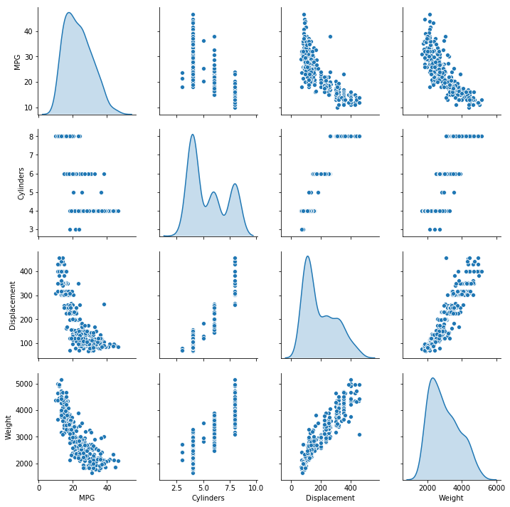
Have a quick look at the joint distribution of a few pairs of columns from the training set.
[12]:
sns.pairplot(train_dataset[["MPG", "Cylinders", "Displacement", "Weight"]], diag_kind="kde")
/anaconda3/lib/python3.6/site-packages/scipy/stats/stats.py:1706: FutureWarning: Using a non-tuple sequence for multidimensional indexing is deprecated; use `arr[tuple(seq)]` instead of `arr[seq]`. In the future this will be interpreted as an array index, `arr[np.array(seq)]`, which will result either in an error or a different result.
  return np.add.reduce(sorted[indexer] * weights, axis=axis) / sumval
[12]:
<seaborn.axisgrid.PairGrid at 0x1348cb128>
Also look at the overall statistics:
[13]:
train_stats = train_dataset.describe()
train_stats.pop("MPG")
train_stats = train_stats.transpose()
train_stats
[13]:
| count | mean | std | min | 25% | 50% | 75% | max | |
|---|---|---|---|---|---|---|---|---|
| Cylinders | 314.0 | 5.477707 | 1.699788 | 3.0 | 4.00 | 4.0 | 8.00 | 8.0 |
| Displacement | 314.0 | 195.318471 | 104.331589 | 68.0 | 105.50 | 151.0 | 265.75 | 455.0 |
| Horsepower | 314.0 | 104.869427 | 38.096214 | 46.0 | 76.25 | 94.5 | 128.00 | 225.0 |
| Weight | 314.0 | 2990.251592 | 843.898596 | 1649.0 | 2256.50 | 2822.5 | 3608.00 | 5140.0 |
| Acceleration | 314.0 | 15.559236 | 2.789230 | 8.0 | 13.80 | 15.5 | 17.20 | 24.8 |
| Model Year | 314.0 | 75.898089 | 3.675642 | 70.0 | 73.00 | 76.0 | 79.00 | 82.0 |
| USA | 314.0 | 0.624204 | 0.485101 | 0.0 | 0.00 | 1.0 | 1.00 | 1.0 |
| Europe | 314.0 | 0.178344 | 0.383413 | 0.0 | 0.00 | 0.0 | 0.00 | 1.0 |
| Japan | 314.0 | 0.197452 | 0.398712 | 0.0 | 0.00 | 0.0 | 0.00 | 1.0 |
Split features from labels
Separate the target value, or “label”, from the features. This label is the value that you will train the model to predict.
[14]:
train_labels = train_dataset.pop('MPG')
test_labels = test_dataset.pop('MPG')
Normalize the data
Look again at the train_stats block above and note how different the ranges of each feature are.
It is good practice to normalize features that use different scales and ranges. Although the model might converge without feature normalization, it makes training more difficult, and it makes the resulting model dependent on the choice of units used in the input.
Note: Although we intentionally generate these statistics from only the training dataset, these statistics will also be used to normalize the test dataset. We need to do that to project the test dataset into the same distribution that the model has been trained on.
[15]:
def norm(x):
  return (x - train_stats['mean']) / train_stats['std']
normed_train_data = norm(train_dataset)
normed_test_data = norm(test_dataset)
This normalized data is what we will use to train the model.
Caution: The statistics used to normalize the inputs here (mean and standard deviation) need to be applied to any other data that is fed to the model, along with the one-hot encoding that we did earlier. That includes the test set as well as live data when the model is used in production.
The model
Build the model
Let’s build our model. Here, we’ll use a Sequential model with two densely connected hidden layers, and an output layer that returns a single, continuous value. The model building steps are wrapped in a function, build_model, since we’ll create a second model, later on.
[16]:
def build_model():
  model = keras.Sequential([
    layers.Dense(64, activation=tf.nn.relu, input_shape=[len(train_dataset.keys())]),
    layers.Dense(64, activation=tf.nn.relu),
    layers.Dense(1)
  ])

  optimizer = tf.keras.optimizers.RMSprop(0.001)

  model.compile(loss='mean_squared_error',
                optimizer=optimizer,
                metrics=['mean_absolute_error', 'mean_squared_error'])
  return model
[17]:
model = build_model()
WARNING:tensorflow:From /anaconda3/lib/python3.6/site-packages/tensorflow/python/ops/resource_variable_ops.py:435: colocate_with (from tensorflow.python.framework.ops) is deprecated and will be removed in a future version.
Instructions for updating:
Colocations handled automatically by placer.
WARNING:tensorflow:From /anaconda3/lib/python3.6/site-packages/tensorflow/python/keras/utils/losses_utils.py:170: to_float (from tensorflow.python.ops.math_ops) is deprecated and will be removed in a future version.
Instructions for updating:
Use tf.cast instead.
Inspect the model
Use the .summary method to print a simple description of the model
[18]:
model.summary()
_________________________________________________________________
Layer (type)                 Output Shape              Param #
=================================================================
dense (Dense)                (None, 64)                640
_________________________________________________________________
dense_1 (Dense)              (None, 64)                4160
_________________________________________________________________
dense_2 (Dense)              (None, 1)                 65
=================================================================
Total params: 4,865
Trainable params: 4,865
Non-trainable params: 0
_________________________________________________________________
Now try out the model. Take a batch of 10 examples from the training data and call model.predict on it.
[19]:
example_batch = normed_train_data[:10]
example_result = model.predict(example_batch)
example_result
[19]:
array([[ 0.07596536],
       [-0.04469106],
       [-0.16783425],
       [ 0.05479676],
       [-0.30215877],
       [-0.04577077],
       [-0.34394804],
       [-0.51477456],
       [-0.0190323 ],
       [ 0.06816971]], dtype=float32)
It seems to be working, and it produces a result of the expected shape and type.
Train the model
Train the model for 1000 epochs, and record the training and validation accuracy in the history object.
[20]:
# Display training progress by printing a single dot for each completed epoch
class PrintDot(keras.callbacks.Callback):
  def on_epoch_end(self, epoch, logs):
    if epoch % 100 == 0: print('')
    print('.', end='')

EPOCHS = 1000

history = model.fit(
  normed_train_data, train_labels,
  epochs=EPOCHS, validation_split = 0.2, verbose=0,
  callbacks=[PrintDot()])
WARNING:tensorflow:From /anaconda3/lib/python3.6/site-packages/tensorflow/python/ops/math_ops.py:3066: to_int32 (from tensorflow.python.ops.math_ops) is deprecated and will be removed in a future version.
Instructions for updating:
Use tf.cast instead.

....................................................................................................
....................................................................................................
....................................................................................................
....................................................................................................
....................................................................................................
....................................................................................................
....................................................................................................
....................................................................................................
....................................................................................................
....................................................................................................
Visualize the model’s training progress using the stats stored in the history object.
[21]:
hist = pd.DataFrame(history.history)
hist['epoch'] = history.epoch
hist.tail()
[21]:
| loss | mean_absolute_error | mean_squared_error | val_loss | val_mean_absolute_error | val_mean_squared_error | epoch | |
|---|---|---|---|---|---|---|---|
| 995 | 2.694101 | 1.087085 | 2.694101 | 8.811951 | 2.326594 | 8.811951 | 995 |
| 996 | 2.615858 | 1.061511 | 2.615858 | 8.505852 | 2.248394 | 8.505852 | 996 |
| 997 | 2.627782 | 1.068165 | 2.627782 | 8.585235 | 2.310220 | 8.585235 | 997 |
| 998 | 2.597472 | 1.016204 | 2.597472 | 9.060644 | 2.373475 | 9.060644 | 998 |
| 999 | 2.619572 | 1.008772 | 2.619571 | 9.023963 | 2.354825 | 9.023963 | 999 |
[22]:
def plot_history(history):
hist = pd.DataFrame(history.history)
hist['epoch'] = history.epoch
plt.figure()
plt.xlabel('Epoch')
plt.ylabel('Mean Abs Error [MPG]')
plt.plot(hist['epoch'], hist['mean_absolute_error'],
label='Train Error')
plt.plot(hist['epoch'], hist['val_mean_absolute_error'],
label = 'Val Error')
plt.ylim([0,5])
plt.legend()
plt.figure()
plt.xlabel('Epoch')
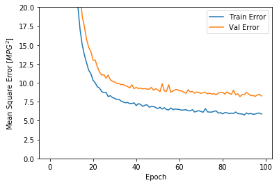
plt.ylabel('Mean Square Error [$MPG^2$]')
plt.plot(hist['epoch'], hist['mean_squared_error'],
label='Train Error')
plt.plot(hist['epoch'], hist['val_mean_squared_error'],
label = 'Val Error')
plt.ylim([0,20])
plt.legend()
plt.show()
plot_history(history)
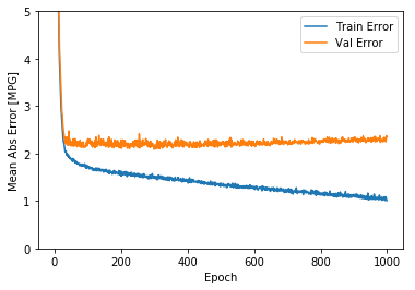
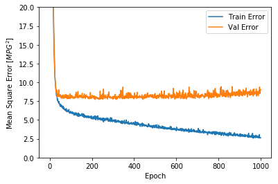
This graph shows little improvement, or even degradation in the validation error after about 100 epochs. Let’s update the model.fit call to automatically stop training when the validation score doesn’t improve. We’ll use an EarlyStopping callback that tests a training condition for every epoch. If a set amount of epochs elapses without showing improvement, then automatically stop the training.
You can learn more about this callback here.
[23]:
model = build_model()

# The patience parameter is the amount of epochs to check for improvement
early_stop = keras.callbacks.EarlyStopping(monitor='val_loss', patience=10)

history = model.fit(normed_train_data, train_labels, epochs=EPOCHS,
                    validation_split = 0.2, verbose=0, callbacks=[early_stop, PrintDot()])

plot_history(history)
...................................................................................................
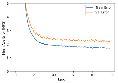
The graph shows that on the validation set, the average error is usually around +/- 2 MPG. Is this good? We’ll leave that decision up to you.
Let’s see how well the model generalizes by using the test set, which we did not use when training the model. This tells us how well we can expect the model to predict when we use it in the real world.
[24]:
loss, mae, mse = model.evaluate(normed_test_data, test_labels, verbose=0)

print("Testing set Mean Abs Error: {:5.2f} MPG".format(mae))
Testing set Mean Abs Error: 1.90 MPG
Make predictions
Finally, predict MPG values using data in the testing set:
[25]:
test_predictions = model.predict(normed_test_data).flatten()

plt.scatter(test_labels, test_predictions)
plt.xlabel('True Values [MPG]')
plt.ylabel('Predictions [MPG]')
plt.axis('equal')
plt.axis('square')
plt.xlim([0,plt.xlim()[1]])
plt.ylim([0,plt.ylim()[1]])
_ = plt.plot([-100, 100], [-100, 100])
It looks like our model predicts reasonably well. Let’s take a look at the error distribution.
[26]:
error = test_predictions - test_labels
plt.hist(error, bins = 25)
plt.xlabel("Prediction Error [MPG]")
_ = plt.ylabel("Count")
It’s not quite gaussian, but we might expect that because the number of samples is very small.
Conclusion
This notebook introduced a few techniques to handle a regression problem.
- Mean Squared Error (MSE) is a common loss function used for regression problems (different loss functions are used for classification problems).
- Similarly, evaluation metrics used for regression differ from classification. A common regression metric is Mean Absolute Error (MAE).
- When numeric input data features have values with different ranges, each feature should be scaled independently to the same range.
- If there is not much training data, one technique is to prefer a small network with few hidden layers to avoid overfitting.
- Early stopping is a useful technique to prevent overfitting.
[ ]: