Copyright 2018 The TensorFlow Authors.
[1]:
#@title Licensed under the Apache License, Version 2.0 (the "License");
# you may not use this file except in compliance with the License.
# You may obtain a copy of the License at
#
# https://www.apache.org/licenses/LICENSE-2.0
#
# Unless required by applicable law or agreed to in writing, software
# distributed under the License is distributed on an "AS IS" BASIS,
# WITHOUT WARRANTIES OR CONDITIONS OF ANY KIND, either express or implied.
# See the License for the specific language governing permissions and
# limitations under the License.
[2]:
#@title MIT License
#
# Copyright (c) 2017 François Chollet
#
# Permission is hereby granted, free of charge, to any person obtaining a
# copy of this software and associated documentation files (the "Software"),
# to deal in the Software without restriction, including without limitation
# the rights to use, copy, modify, merge, publish, distribute, sublicense,
# and/or sell copies of the Software, and to permit persons to whom the
# Software is furnished to do so, subject to the following conditions:
#
# The above copyright notice and this permission notice shall be included in
# all copies or substantial portions of the Software.
#
# THE SOFTWARE IS PROVIDED "AS IS", WITHOUT WARRANTY OF ANY KIND, EXPRESS OR
# IMPLIED, INCLUDING BUT NOT LIMITED TO THE WARRANTIES OF MERCHANTABILITY,
# FITNESS FOR A PARTICULAR PURPOSE AND NONINFRINGEMENT. IN NO EVENT SHALL
# THE AUTHORS OR COPYRIGHT HOLDERS BE LIABLE FOR ANY CLAIM, DAMAGES OR OTHER
# LIABILITY, WHETHER IN AN ACTION OF CONTRACT, TORT OR OTHERWISE, ARISING
# FROM, OUT OF OR IN CONNECTION WITH THE SOFTWARE OR THE USE OR OTHER
# DEALINGS IN THE SOFTWARE.
Text classification with movie reviews
<a target="_blank" href="https://www.tensorflow.org/tutorials/keras/basic_text_classification"><img src="https://www.tensorflow.org/images/tf_logo_32px.png" />View on TensorFlow.org</a>
| <a target="_blank" href="https://colab.research.google.com/github/tensorflow/docs/blob/master/site/en/tutorials/keras/basic_text_classification.ipynb"><img src="https://www.tensorflow.org/images/colab_logo_32px.png" />Run in Google Colab</a>
| <a target="_blank" href="https://github.com/tensorflow/docs/blob/master/site/en/tutorials/keras/basic_text_classification.ipynb"><img src="https://www.tensorflow.org/images/GitHub-Mark-32px.png" />View source on GitHub</a>
|
This notebook classifies movie reviews as positive or negative using the text of the review. This is an example of binary—or two-class—classification, an important and widely applicable kind of machine learning problem.
We’ll use the IMDB dataset that contains the text of 50,000 movie reviews from the Internet Movie Database. These are split into 25,000 reviews for training and 25,000 reviews for testing. The training and testing sets are balanced, meaning they contain an equal number of positive and negative reviews.
This notebook uses tf.keras, a high-level API to build and train models in TensorFlow. For a more advanced text classification tutorial using tf.keras, see the MLCC Text Classification Guide.
[3]:
# keras.datasets.imdb is broken in 1.13 and 1.14, by np 1.16.3
!pip install tf_nightly
Collecting tf_nightly
  Downloading https://files.pythonhosted.org/packages/f6/b8/1383cdc340f142a0a8439a7ec171c733f998c7dfaceab1ccc27bcb4cd4af/tf_nightly-1.14.1.dev20190607-cp36-cp36m-macosx_10_9_x86_64.whl (103.8MB)
    100% |████████████████████████████████| 103.8MB 478kB/s
Requirement already satisfied: keras-preprocessing>=1.0.5 in /anaconda3/lib/python3.6/site-packages (from tf_nightly) (1.1.0)
Requirement already satisfied: gast>=0.2.0 in /anaconda3/lib/python3.6/site-packages (from tf_nightly) (0.2.0)
Requirement already satisfied: astor>=0.6.0 in /anaconda3/lib/python3.6/site-packages (from tf_nightly) (0.6.2)
Collecting tb-nightly<1.15.0a0,>=1.14.0a0 (from tf_nightly)
  Downloading https://files.pythonhosted.org/packages/9b/df/7d93182f298cdb84d1a219d26f01b4265cea0c2e24a1d09a6f5da7ab4edb/tb_nightly-1.14.0a20190610-py3-none-any.whl (3.1MB)
    100% |████████████████████████████████| 3.2MB 3.4MB/s
Collecting wrapt>=1.11.1 (from tf_nightly)
  Downloading https://files.pythonhosted.org/packages/67/b2/0f71ca90b0ade7fad27e3d20327c996c6252a2ffe88f50a95bba7434eda9/wrapt-1.11.1.tar.gz
Collecting google-pasta>=0.1.6 (from tf_nightly)
  Downloading https://files.pythonhosted.org/packages/d0/33/376510eb8d6246f3c30545f416b2263eee461e40940c2a4413c711bdf62d/google_pasta-0.1.7-py3-none-any.whl (52kB)
    100% |████████████████████████████████| 61kB 5.7MB/s
Requirement already satisfied: termcolor>=1.1.0 in /anaconda3/lib/python3.6/site-packages (from tf_nightly) (1.1.0)
Requirement already satisfied: protobuf>=3.6.1 in /anaconda3/lib/python3.6/site-packages (from tf_nightly) (3.8.0)
Collecting absl-py>=0.7.0 (from tf_nightly)
  Downloading https://files.pythonhosted.org/packages/da/3f/9b0355080b81b15ba6a9ffcf1f5ea39e307a2778b2f2dc8694724e8abd5b/absl-py-0.7.1.tar.gz (99kB)
    100% |████████████████████████████████| 102kB 5.6MB/s
Requirement already satisfied: numpy<2.0,>=1.14.5 in /anaconda3/lib/python3.6/site-packages (from tf_nightly) (1.16.2)
Requirement already satisfied: grpcio>=1.8.6 in /anaconda3/lib/python3.6/site-packages (from tf_nightly) (1.10.0)
Requirement already satisfied: six>=1.10.0 in /anaconda3/lib/python3.6/site-packages (from tf_nightly) (1.12.0)
Requirement already satisfied: wheel>=0.26 in /anaconda3/lib/python3.6/site-packages (from tf_nightly) (0.30.0)
Collecting tf-estimator-nightly (from tf_nightly)
  Downloading https://files.pythonhosted.org/packages/31/ff/9338ea271d0ee5fbb62d267d9dbc4840697e8fe7d8bb70666ead951a13f7/tf_estimator_nightly-1.14.0.dev2019061001-py2.py3-none-any.whl (495kB)
    100% |████████████████████████████████| 501kB 1.7MB/s
Requirement already satisfied: keras-applications>=1.0.6 in /anaconda3/lib/python3.6/site-packages (from tf_nightly) (1.0.8)
Requirement already satisfied: werkzeug>=0.11.15 in /anaconda3/lib/python3.6/site-packages (from tb-nightly<1.15.0a0,>=1.14.0a0->tf_nightly) (0.14.1)
Collecting setuptools>=41.0.0 (from tb-nightly<1.15.0a0,>=1.14.0a0->tf_nightly)
  Using cached https://files.pythonhosted.org/packages/ec/51/f45cea425fd5cb0b0380f5b0f048ebc1da5b417e48d304838c02d6288a1e/setuptools-41.0.1-py2.py3-none-any.whl
Requirement already satisfied: markdown>=2.6.8 in /anaconda3/lib/python3.6/site-packages (from tb-nightly<1.15.0a0,>=1.14.0a0->tf_nightly) (2.6.11)
Requirement already satisfied: h5py in /anaconda3/lib/python3.6/site-packages (from keras-applications>=1.0.6->tf_nightly) (2.7.1)
Building wheels for collected packages: wrapt, absl-py
  Building wheel for wrapt (setup.py) ... done
  Stored in directory: /Users/koehlejf/Library/Caches/pip/wheels/89/67/41/63cbf0f6ac0a6156588b9587be4db5565f8c6d8ccef98202fc
  Building wheel for absl-py (setup.py) ... done
  Stored in directory: /Users/koehlejf/Library/Caches/pip/wheels/ee/98/38/46cbcc5a93cfea5492d19c38562691ddb23b940176c14f7b48
Successfully built wrapt absl-py
scrapy 1.5.0 requires pyOpenSSL, which is not installed.
Installing collected packages: setuptools, absl-py, tb-nightly, wrapt, google-pasta, tf-estimator-nightly, tf-nightly
  Found existing installation: setuptools 38.4.0
    Uninstalling setuptools-38.4.0:
      Successfully uninstalled setuptools-38.4.0
  Found existing installation: absl-py 0.1.11
    Uninstalling absl-py-0.1.11:
      Successfully uninstalled absl-py-0.1.11
  Found existing installation: wrapt 1.10.11
Cannot uninstall 'wrapt'. It is a distutils installed project and thus we cannot accurately determine which files belong to it which would lead to only a partial uninstall.
You are using pip version 19.0.3, however version 19.1.1 is available.
You should consider upgrading via the 'pip install --upgrade pip' command.
[4]:
from __future__ import absolute_import, division, print_function, unicode_literals

import tensorflow as tf
from tensorflow import keras

import numpy as np

print(tf.__version__)
/anaconda3/lib/python3.6/site-packages/h5py/__init__.py:36: FutureWarning: Conversion of the second argument of issubdtype from `float` to `np.floating` is deprecated. In future, it will be treated as `np.float64 == np.dtype(float).type`.
  from ._conv import register_converters as _register_converters
1.13.1
Download the IMDB dataset
The IMDB dataset comes packaged with TensorFlow. It has already been preprocessed such that the reviews (sequences of words) have been converted to sequences of integers, where each integer represents a specific word in a dictionary.
The following code downloads the IMDB dataset to your machine (or uses a cached copy if you’ve already downloaded it):
[5]:
imdb = keras.datasets.imdb

(train_data, train_labels), (test_data, test_labels) = imdb.load_data(num_words=10000)
The argument num_words=10000 keeps the top 10,000 most frequently occurring words in the training data. The rare words are discarded to keep the size of the data manageable.
Explore the data
Let’s take a moment to understand the format of the data. The dataset comes preprocessed: each example is an array of integers representing the words of the movie review. Each label is an integer value of either 0 or 1, where 0 is a negative review, and 1 is a positive review.
[6]:
print("Training entries: {}, labels: {}".format(len(train_data), len(train_labels)))
Training entries: 25000, labels: 25000
The text of reviews have been converted to integers, where each integer represents a specific word in a dictionary. Here’s what the first review looks like:
[7]:
print(train_data[0])
[1, 14, 22, 16, 43, 530, 973, 1622, 1385, 65, 458, 4468, 66, 3941, 4, 173, 36, 256, 5, 25, 100, 43, 838, 112, 50, 670, 2, 9, 35, 480, 284, 5, 150, 4, 172, 112, 167, 2, 336, 385, 39, 4, 172, 4536, 1111, 17, 546, 38, 13, 447, 4, 192, 50, 16, 6, 147, 2025, 19, 14, 22, 4, 1920, 4613, 469, 4, 22, 71, 87, 12, 16, 43, 530, 38, 76, 15, 13, 1247, 4, 22, 17, 515, 17, 12, 16, 626, 18, 2, 5, 62, 386, 12, 8, 316, 8, 106, 5, 4, 2223, 5244, 16, 480, 66, 3785, 33, 4, 130, 12, 16, 38, 619, 5, 25, 124, 51, 36, 135, 48, 25, 1415, 33, 6, 22, 12, 215, 28, 77, 52, 5, 14, 407, 16, 82, 2, 8, 4, 107, 117, 5952, 15, 256, 4, 2, 7, 3766, 5, 723, 36, 71, 43, 530, 476, 26, 400, 317, 46, 7, 4, 2, 1029, 13, 104, 88, 4, 381, 15, 297, 98, 32, 2071, 56, 26, 141, 6, 194, 7486, 18, 4, 226, 22, 21, 134, 476, 26, 480, 5, 144, 30, 5535, 18, 51, 36, 28, 224, 92, 25, 104, 4, 226, 65, 16, 38, 1334, 88, 12, 16, 283, 5, 16, 4472, 113, 103, 32, 15, 16, 5345, 19, 178, 32]
Movie reviews may be different lengths. The below code shows the number of words in the first and second reviews. Since inputs to a neural network must be the same length, we’ll need to resolve this later.
[8]:
len(train_data[0]), len(train_data[1])
[8]:
(218, 189)
Convert the integers back to words
It may be useful to know how to convert integers back to text. Here, we’ll create a helper function to query a dictionary object that contains the integer to string mapping:
[9]:
# A dictionary mapping words to an integer index
word_index = imdb.get_word_index()

# The first indices are reserved
word_index = {k:(v+3) for k,v in word_index.items()}
word_index["<PAD>"] = 0
word_index["<START>"] = 1
word_index["<UNK>"] = 2  # unknown
word_index["<UNUSED>"] = 3

reverse_word_index = dict([(value, key) for (key, value) in word_index.items()])

def decode_review(text):
    return ' '.join([reverse_word_index.get(i, '?') for i in text])
Downloading data from https://storage.googleapis.com/tensorflow/tf-keras-datasets/imdb_word_index.json
1646592/1641221 [==============================] - 1s 0us/step
Now we can use the decode_review function to display the text for the first review:
[10]:
decode_review(train_data[0])
[10]:
"<START> this film was just brilliant casting location scenery story direction everyone's really suited the part they played and you could just imagine being there robert <UNK> is an amazing actor and now the same being director <UNK> father came from the same scottish island as myself so i loved the fact there was a real connection with this film the witty remarks throughout the film were great it was just brilliant so much that i bought the film as soon as it was released for <UNK> and would recommend it to everyone to watch and the fly fishing was amazing really cried at the end it was so sad and you know what they say if you cry at a film it must have been good and this definitely was also <UNK> to the two little boy's that played the <UNK> of norman and paul they were just brilliant children are often left out of the <UNK> list i think because the stars that play them all grown up are such a big profile for the whole film but these children are amazing and should be praised for what they have done don't you think the whole story was so lovely because it was true and was someone's life after all that was shared with us all"
Prepare the data
The reviews—the arrays of integers—must be converted to tensors before fed into the neural network. This conversion can be done a couple of ways:
- Convert the arrays into vectors of 0s and 1s indicating word occurrence, similar to a one-hot encoding. For example, the sequence [3, 5] would become a 10,000-dimensional vector that is all zeros except for indices 3 and 5, which are ones. Then, make this the first layer in our network—a Dense layer—that can handle floating point vector data. This approach is memory intensive, though, requiring a
num_words * num_reviewssize matrix. - Alternatively, we can pad the arrays so they all have the same length, then create an integer tensor of shape
max_length * num_reviews. We can use an embedding layer capable of handling this shape as the first layer in our network.
In this tutorial, we will use the second approach.
Since the movie reviews must be the same length, we will use the pad_sequences function to standardize the lengths:
[11]:
train_data = keras.preprocessing.sequence.pad_sequences(train_data,
                                                        value=word_index["<PAD>"],
                                                        padding='post',
                                                        maxlen=256)

test_data = keras.preprocessing.sequence.pad_sequences(test_data,
                                                       value=word_index["<PAD>"],
                                                       padding='post',
                                                       maxlen=256)
Let’s look at the length of the examples now:
[12]:
len(train_data[0]), len(train_data[1])
[12]:
(256, 256)
And inspect the (now padded) first review:
[13]:
print(train_data[0])
[   1   14   22   16   43  530  973 1622 1385   65  458 4468   66 3941
    4  173   36  256    5   25  100   43  838  112   50  670    2    9
   35  480  284    5  150    4  172  112  167    2  336  385   39    4
  172 4536 1111   17  546   38   13  447    4  192   50   16    6  147
 2025   19   14   22    4 1920 4613  469    4   22   71   87   12   16
   43  530   38   76   15   13 1247    4   22   17  515   17   12   16
  626   18    2    5   62  386   12    8  316    8  106    5    4 2223
 5244   16  480   66 3785   33    4  130   12   16   38  619    5   25
  124   51   36  135   48   25 1415   33    6   22   12  215   28   77
   52    5   14  407   16   82    2    8    4  107  117 5952   15  256
    4    2    7 3766    5  723   36   71   43  530  476   26  400  317
   46    7    4    2 1029   13  104   88    4  381   15  297   98   32
 2071   56   26  141    6  194 7486   18    4  226   22   21  134  476
   26  480    5  144   30 5535   18   51   36   28  224   92   25  104
    4  226   65   16   38 1334   88   12   16  283    5   16 4472  113
  103   32   15   16 5345   19  178   32    0    0    0    0    0    0
    0    0    0    0    0    0    0    0    0    0    0    0    0    0
    0    0    0    0    0    0    0    0    0    0    0    0    0    0
    0    0    0    0]
Build the model
The neural network is created by stacking layers—this requires two main architectural decisions:
- How many layers to use in the model?
- How many hidden units to use for each layer?
In this example, the input data consists of an array of word-indices. The labels to predict are either 0 or 1. Let’s build a model for this problem:
[14]:
# input shape is the vocabulary count used for the movie reviews (10,000 words)
vocab_size = 10000

model = keras.Sequential()
model.add(keras.layers.Embedding(vocab_size, 16))
model.add(keras.layers.GlobalAveragePooling1D())
model.add(keras.layers.Dense(16, activation=tf.nn.relu))
model.add(keras.layers.Dense(1, activation=tf.nn.sigmoid))

model.summary()
WARNING:tensorflow:From /anaconda3/lib/python3.6/site-packages/tensorflow/python/ops/resource_variable_ops.py:435: colocate_with (from tensorflow.python.framework.ops) is deprecated and will be removed in a future version.
Instructions for updating:
Colocations handled automatically by placer.
_________________________________________________________________
Layer (type)                 Output Shape              Param #
=================================================================
embedding (Embedding)        (None, None, 16)          160000
_________________________________________________________________
global_average_pooling1d (Gl (None, 16)                0
_________________________________________________________________
dense (Dense)                (None, 16)                272
_________________________________________________________________
dense_1 (Dense)              (None, 1)                 17
=================================================================
Total params: 160,289
Trainable params: 160,289
Non-trainable params: 0
_________________________________________________________________
The layers are stacked sequentially to build the classifier:
- The first layer is an
Embeddinglayer. This layer takes the integer-encoded vocabulary and looks up the embedding vector for each word-index. These vectors are learned as the model trains. The vectors add a dimension to the output array. The resulting dimensions are:(batch, sequence, embedding). - Next, a
GlobalAveragePooling1Dlayer returns a fixed-length output vector for each example by averaging over the sequence dimension. This allows the model to handle input of variable length, in the simplest way possible. - This fixed-length output vector is piped through a fully-connected (
Dense) layer with 16 hidden units. - The last layer is densely connected with a single output node. Using the
sigmoidactivation function, this value is a float between 0 and 1, representing a probability, or confidence level.
Hidden units
The above model has two intermediate or “hidden” layers, between the input and output. The number of outputs (units, nodes, or neurons) is the dimension of the representational space for the layer. In other words, the amount of freedom the network is allowed when learning an internal representation.
If a model has more hidden units (a higher-dimensional representation space), and/or more layers, then the network can learn more complex representations. However, it makes the network more computationally expensive and may lead to learning unwanted patterns—patterns that improve performance on training data but not on the test data. This is called overfitting, and we’ll explore it later.
Loss function and optimizer
A model needs a loss function and an optimizer for training. Since this is a binary classification problem and the model outputs a probability (a single-unit layer with a sigmoid activation), we’ll use the binary_crossentropy loss function.
This isn’t the only choice for a loss function, you could, for instance, choose mean_squared_error. But, generally, binary_crossentropy is better for dealing with probabilities—it measures the “distance” between probability distributions, or in our case, between the ground-truth distribution and the predictions.
Later, when we are exploring regression problems (say, to predict the price of a house), we will see how to use another loss function called mean squared error.
Now, configure the model to use an optimizer and a loss function:
[15]:
model.compile(optimizer='adam',
              loss='binary_crossentropy',
              metrics=['acc'])
Create a validation set
When training, we want to check the accuracy of the model on data it hasn’t seen before. Create a validation set by setting apart 10,000 examples from the original training data. (Why not use the testing set now? Our goal is to develop and tune our model using only the training data, then use the test data just once to evaluate our accuracy).
[16]:
x_val = train_data[:10000]
partial_x_train = train_data[10000:]

y_val = train_labels[:10000]
partial_y_train = train_labels[10000:]
Train the model
Train the model for 40 epochs in mini-batches of 512 samples. This is 40 iterations over all samples in the x_train and y_train tensors. While training, monitor the model’s loss and accuracy on the 10,000 samples from the validation set:
[17]:
history = model.fit(partial_x_train,
                    partial_y_train,
                    epochs=40,
                    batch_size=512,
                    validation_data=(x_val, y_val),
                    verbose=1)
Train on 15000 samples, validate on 10000 samples
WARNING:tensorflow:From /anaconda3/lib/python3.6/site-packages/tensorflow/python/ops/math_ops.py:3066: to_int32 (from tensorflow.python.ops.math_ops) is deprecated and will be removed in a future version.
Instructions for updating:
Use tf.cast instead.
Epoch 1/40
15000/15000 [==============================] - 1s 40us/sample - loss: 0.6920 - acc: 0.5314 - val_loss: 0.6902 - val_acc: 0.5870
Epoch 2/40
15000/15000 [==============================] - 0s 21us/sample - loss: 0.6867 - acc: 0.6896 - val_loss: 0.6831 - val_acc: 0.7147
Epoch 3/40
15000/15000 [==============================] - 0s 21us/sample - loss: 0.6748 - acc: 0.7326 - val_loss: 0.6676 - val_acc: 0.7505
Epoch 4/40
15000/15000 [==============================] - 0s 21us/sample - loss: 0.6535 - acc: 0.7485 - val_loss: 0.6436 - val_acc: 0.7618
Epoch 5/40
15000/15000 [==============================] - 0s 21us/sample - loss: 0.6225 - acc: 0.7826 - val_loss: 0.6113 - val_acc: 0.7824
Epoch 6/40
15000/15000 [==============================] - 0s 21us/sample - loss: 0.5831 - acc: 0.8060 - val_loss: 0.5735 - val_acc: 0.7972
Epoch 7/40
15000/15000 [==============================] - 0s 21us/sample - loss: 0.5388 - acc: 0.8250 - val_loss: 0.5315 - val_acc: 0.8188
Epoch 8/40
15000/15000 [==============================] - 0s 22us/sample - loss: 0.4937 - acc: 0.8445 - val_loss: 0.4920 - val_acc: 0.8296
Epoch 9/40
15000/15000 [==============================] - 0s 22us/sample - loss: 0.4510 - acc: 0.8583 - val_loss: 0.4554 - val_acc: 0.8412
Epoch 10/40
15000/15000 [==============================] - 0s 21us/sample - loss: 0.4123 - acc: 0.8720 - val_loss: 0.4246 - val_acc: 0.8484
Epoch 11/40
15000/15000 [==============================] - 0s 21us/sample - loss: 0.3790 - acc: 0.8791 - val_loss: 0.3983 - val_acc: 0.8573
Epoch 12/40
15000/15000 [==============================] - 0s 21us/sample - loss: 0.3505 - acc: 0.8874 - val_loss: 0.3781 - val_acc: 0.8594
Epoch 13/40
15000/15000 [==============================] - 0s 21us/sample - loss: 0.3269 - acc: 0.8935 - val_loss: 0.3597 - val_acc: 0.8663
Epoch 14/40
15000/15000 [==============================] - 0s 20us/sample - loss: 0.3056 - acc: 0.8991 - val_loss: 0.3463 - val_acc: 0.8710
Epoch 15/40
15000/15000 [==============================] - 0s 20us/sample - loss: 0.2880 - acc: 0.9032 - val_loss: 0.3347 - val_acc: 0.8730
Epoch 16/40
15000/15000 [==============================] - 0s 20us/sample - loss: 0.2721 - acc: 0.9082 - val_loss: 0.3254 - val_acc: 0.8748
Epoch 17/40
15000/15000 [==============================] - 0s 21us/sample - loss: 0.2576 - acc: 0.9133 - val_loss: 0.3175 - val_acc: 0.8774
Epoch 18/40
15000/15000 [==============================] - 0s 21us/sample - loss: 0.2447 - acc: 0.9173 - val_loss: 0.3104 - val_acc: 0.8800
Epoch 19/40
15000/15000 [==============================] - 0s 21us/sample - loss: 0.2331 - acc: 0.9203 - val_loss: 0.3048 - val_acc: 0.8801
Epoch 20/40
15000/15000 [==============================] - 0s 22us/sample - loss: 0.2226 - acc: 0.9240 - val_loss: 0.3007 - val_acc: 0.8806
Epoch 21/40
15000/15000 [==============================] - 0s 23us/sample - loss: 0.2121 - acc: 0.9289 - val_loss: 0.2973 - val_acc: 0.8812
Epoch 22/40
15000/15000 [==============================] - 0s 21us/sample - loss: 0.2033 - acc: 0.9309 - val_loss: 0.2936 - val_acc: 0.8844
Epoch 23/40
15000/15000 [==============================] - 0s 21us/sample - loss: 0.1943 - acc: 0.9347 - val_loss: 0.2919 - val_acc: 0.8833
Epoch 24/40
15000/15000 [==============================] - 0s 20us/sample - loss: 0.1866 - acc: 0.9386 - val_loss: 0.2901 - val_acc: 0.8851
Epoch 25/40
15000/15000 [==============================] - 0s 20us/sample - loss: 0.1787 - acc: 0.9429 - val_loss: 0.2877 - val_acc: 0.8845
Epoch 26/40
15000/15000 [==============================] - 0s 21us/sample - loss: 0.1716 - acc: 0.9451 - val_loss: 0.2879 - val_acc: 0.8839
Epoch 27/40
15000/15000 [==============================] - 0s 20us/sample - loss: 0.1650 - acc: 0.9475 - val_loss: 0.2867 - val_acc: 0.8839
Epoch 28/40
15000/15000 [==============================] - 0s 20us/sample - loss: 0.1585 - acc: 0.9509 - val_loss: 0.2869 - val_acc: 0.8846
Epoch 29/40
15000/15000 [==============================] - 0s 21us/sample - loss: 0.1530 - acc: 0.9539 - val_loss: 0.2873 - val_acc: 0.8835
Epoch 30/40
15000/15000 [==============================] - 0s 21us/sample - loss: 0.1471 - acc: 0.9547 - val_loss: 0.2866 - val_acc: 0.8864
Epoch 31/40
15000/15000 [==============================] - 0s 22us/sample - loss: 0.1412 - acc: 0.9587 - val_loss: 0.2870 - val_acc: 0.8862
Epoch 32/40
15000/15000 [==============================] - 0s 21us/sample - loss: 0.1359 - acc: 0.9607 - val_loss: 0.2880 - val_acc: 0.8854
Epoch 33/40
15000/15000 [==============================] - 0s 21us/sample - loss: 0.1307 - acc: 0.9622 - val_loss: 0.2897 - val_acc: 0.8864
Epoch 34/40
15000/15000 [==============================] - 0s 20us/sample - loss: 0.1261 - acc: 0.9637 - val_loss: 0.2914 - val_acc: 0.8854
Epoch 35/40
15000/15000 [==============================] - 0s 20us/sample - loss: 0.1219 - acc: 0.9643 - val_loss: 0.2928 - val_acc: 0.8860
Epoch 36/40
15000/15000 [==============================] - 0s 20us/sample - loss: 0.1173 - acc: 0.9671 - val_loss: 0.2942 - val_acc: 0.8855
Epoch 37/40
15000/15000 [==============================] - 0s 20us/sample - loss: 0.1128 - acc: 0.9688 - val_loss: 0.2965 - val_acc: 0.8846
Epoch 38/40
15000/15000 [==============================] - 0s 20us/sample - loss: 0.1087 - acc: 0.9705 - val_loss: 0.2993 - val_acc: 0.8837
Epoch 39/40
15000/15000 [==============================] - 0s 20us/sample - loss: 0.1055 - acc: 0.9711 - val_loss: 0.3024 - val_acc: 0.8835
Epoch 40/40
15000/15000 [==============================] - 0s 20us/sample - loss: 0.1013 - acc: 0.9732 - val_loss: 0.3045 - val_acc: 0.8843
Evaluate the model
And let’s see how the model performs. Two values will be returned. Loss (a number which represents our error, lower values are better), and accuracy.
[18]:
results = model.evaluate(test_data, test_labels)

print(results)
25000/25000 [==============================] - 0s 14us/sample - loss: 0.3243 - acc: 0.8719
[0.32434944102287294, 0.87192]
This fairly naive approach achieves an accuracy of about 87%. With more advanced approaches, the model should get closer to 95%.
Create a graph of accuracy and loss over time
model.fit() returns a History object that contains a dictionary with everything that happened during training:
[19]:
history_dict = history.history
history_dict.keys()
[19]:
dict_keys(['loss', 'acc', 'val_loss', 'val_acc'])
There are four entries: one for each monitored metric during training and validation. We can use these to plot the training and validation loss for comparison, as well as the training and validation accuracy:
[20]:
import matplotlib.pyplot as plt
acc = history_dict['acc']
val_acc = history_dict['val_acc']
loss = history_dict['loss']
val_loss = history_dict['val_loss']
epochs = range(1, len(acc) + 1)
# "bo" is for "blue dot"
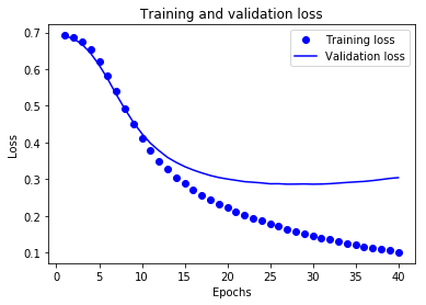
plt.plot(epochs, loss, 'bo', label='Training loss')
# b is for "solid blue line"
plt.plot(epochs, val_loss, 'b', label='Validation loss')
plt.title('Training and validation loss')
plt.xlabel('Epochs')
plt.ylabel('Loss')
plt.legend()
plt.show()
[21]:
plt.clf()   # clear figure

plt.plot(epochs, acc, 'bo', label='Training acc')
plt.plot(epochs, val_acc, 'b', label='Validation acc')
plt.title('Training and validation accuracy')
plt.xlabel('Epochs')
plt.ylabel('Accuracy')
plt.legend()

plt.show()
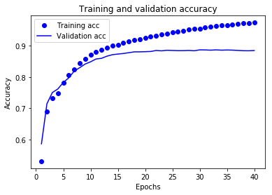
In this plot, the dots represent the training loss and accuracy, and the solid lines are the validation loss and accuracy.
Notice the training loss decreases with each epoch and the training accuracy increases with each epoch. This is expected when using a gradient descent optimization—it should minimize the desired quantity on every iteration.
This isn’t the case for the validation loss and accuracy—they seem to peak after about twenty epochs. This is an example of overfitting: the model performs better on the training data than it does on data it has never seen before. After this point, the model over-optimizes and learns representations specific to the training data that do not generalize to test data.
For this particular case, we could prevent overfitting by simply stopping the training after twenty or so epochs. Later, you’ll see how to do this automatically with a callback.
[ ]: